关于Fashion Mnist数据集不同训练方法的总结

• 导航
  • 数据输入与处理
  • 训练函数与评估函数
  • Softmax回归
  • MLP
  • MLP + 权重衰减
    • 权重衰减
  • MLP + dropout
  • 附录
  • Reference

本文所有的训练方法都是把输入展平成一维向量做的，所以容易损失很多空间信息，准确度并不高

先给大家看看结果，这是20个epoch的

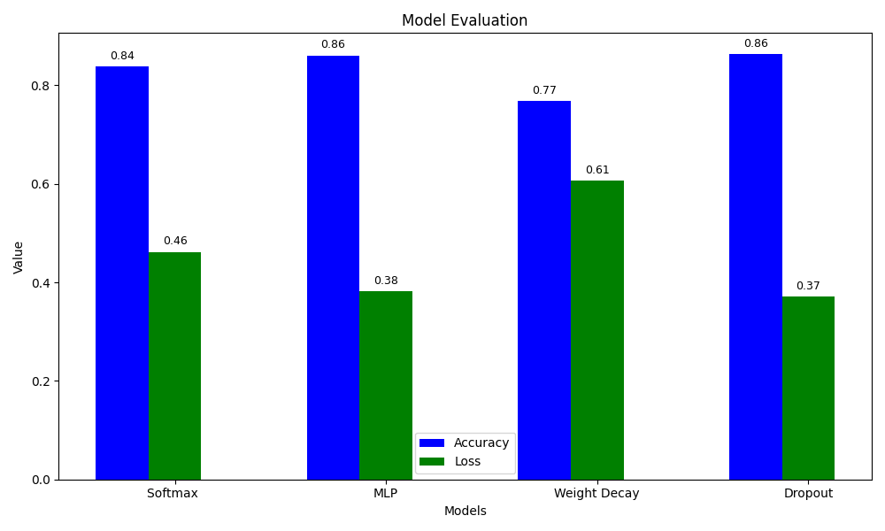
其实能看到差别不大。。

其实也许是因为展平之后损失的信息没法找补回来吧。但是能看到，dropout的loss是最低的，它表现的最好

还能发现权重衰减只有0.7几，我感觉是我参数没调好

我的参数

    batch_size, lr, num_epochs, num_inputs, num_hidden, num_outputs = 256, 0.1, 20, 784, 256, 10
    num_hidden2 = 256
    p=0.5
    lambd = 0.01

后来我把参数调成

    batch_size, lr, num_epochs, num_inputs, num_hidden, num_outputs = 256, 0.1, 30, 784, 256, 10
    num_hidden2 = 256
    p=0.5
    lambd = 0.0005

跑30epoch

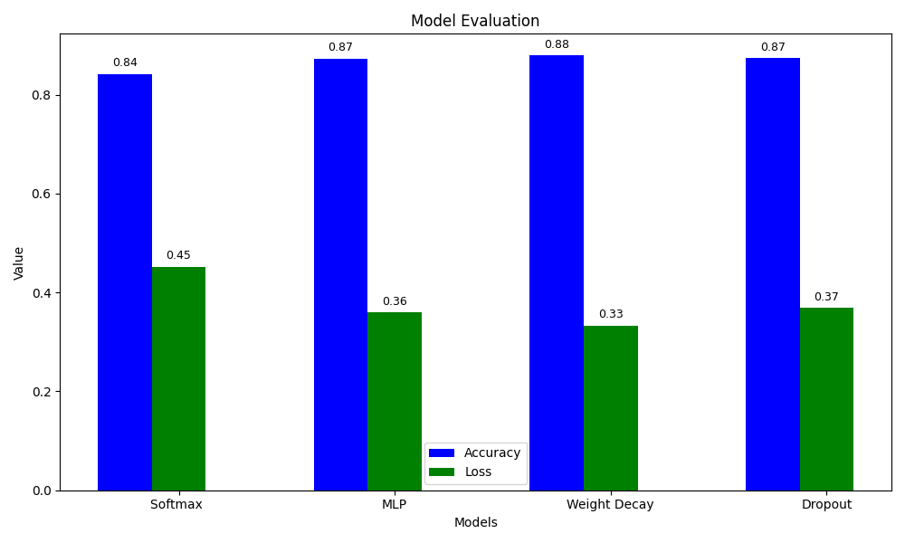
能发现好很多了，前面推测是$\lambda$太大导致惩罚太高。

这样看起来似乎除了softmax差一点之外，其它几个模型没什么大差距，可能是这个训练集比较简单

数据输入与处理

def get_dataloader_workers():
    return 4

def load_data_fashion_minst(batch_size, resize=None):
    trans = [
        transforms.ToTensor(),
        #transforms.Lambda(lambda x : x.view(-1))
    ]
    if resize:
        if isinstance(resize, (tuple, int)):
            trans.insert(0, transforms.Resize(resize))  # type: ignore
        else:
            raise ValueError(
                "resize must be an integer or a tuple of integers")
    trans = transforms.Compose(trans)
    #    print(trans)
    mnist_train = torchvision.datasets.FashionMNIST(root="data",
                                                    train=True,
                                                    transform=trans,
                                                    download=True)
    mnist_test = torchvision.datasets.FashionMNIST(root="data",
                                                   train=False,
                                                   transform=trans,
                                                   download=True)
    return (data.DataLoader(mnist_train,
                            batch_size,
                            shuffle=True,
                            num_workers=get_dataloader_workers()),
            data.DataLoader(mnist_test,
                            batch_size,
                            shuffle=False,
                            num_workers=get_dataloader_workers()))

由于展平操作在net里面做了，所以这里的trans只有一个totenser，把图片变成向量。然后用dataloader返回两个迭代器，分别是训练集和测试集

注意，如果你的num_workers不是0，并且是windows的话，记得写个main函数，不然会报错

训练函数与评估函数

def train_net(net, train_iter, num_epochs, loss, trainer,test_iter):
    print(f"Training {net.__class__.__name__}...")
    timer=0

    epoch_losses = []
#    epoch_accs = []
    test_losses = []
    if isinstance(net, nn.Module):
        net.train()
    for epoch in range(num_epochs):
        metric = Accumulator(3)  # Sum of loss, accuracy and total number of predictions
        for X, y in train_iter:
                start_time = time.time()
                X, y = X.to(next(net.parameters()).device), y.to(next(net.parameters()).device)
                y_hat = net(X)
                l = loss(y_hat, y).mean()
                trainer.zero_grad()
                l.backward()
                trainer.step()
                end_time = time.time()
                timer += end_time - start_time
                # 记录损失和准确率
                metric.add(l.item() * y.size(0), d2l.accuracy(y_hat, y), y.size(0))
                epoch_loss = metric[0] / metric[2]
        epoch_loss = metric[0] / metric[2]
#        epoch_acc = metric[1] / metric[2]
        epoch_losses.append(epoch_loss)
        epoch_accs.append(epoch_acc)
        test_losses.append(evaluate_loss(net,test_iter,loss))

    return timer, epoch_losses, test_losses

其它杂七杂八的都可以不用看，是我用来记录数据的，核心就这几句

                y_hat = net(X)
                l = loss(y_hat, y).mean()
                trainer.zero_grad()
                l.backward()
                trainer.step()
                end_time = time.time()
                timer += end_time - start_time

然后是评估函数

def evaluate_accuracy(net, test_iter):
    if isinstance(net, torch.nn.Module):
        net.eval()
    metric = Accumulator(
        2)  # Sum of correct predictions and total number of predictions
    with torch.no_grad():
        for X, y in test_iter:
            X, y = X.to(next(net.parameters()).device), y.to(
                next(net.parameters()).device)
            metric.add(d2l.accuracy(net(X), y), y.numel())
    return metric[0] / metric[1]

def evaluate_loss(net, test_iter, loss):
    if isinstance(net, nn.Module):
        net.eval()
    metric = Accumulator(2)  # Sum of loss and total number of predictions
    with torch.no_grad():
        for X, y in test_iter:
            X, y = X.to(next(net.parameters()).device), y.to(
                next(net.parameters()).device)
            metric.add(loss(net(X), y).sum(), y.numel())
    return metric[0] / metric[1]

Accumulator是我自己定义的一个类(其实是抄的d2l上面的),就是用来计数的

class Accumulator:

    def __init__(self, n):
        self.data = [0.0] * n

    def add(self, *args):
        self.data = [a + float(b) for a, b in zip(self.data, args)]

    def __getitem__(self, idx):
        return self.data[idx]

Softmax回归

Softmax回归是一个线性模型，由于我们把输入的图像从28 28展平成了1 784，所以其实我们的函数就是一个很简单的线性模型
$$
y=WX^T+b
$$
其中y是10 1的向量(总共有10个种类的服装)，W是10 784，X是1 784的向量，b是10 1的向量。其实就是十个输出，每个输出都有一个线性函数来拟合

对于一个分类问题，我们希望输出的是一个概率，但是我们不能保证线性模型的输出符合要求，怎么办呢？我们需要使用softmax函数来整理我们的输出
$$
softmax(x_i)=\frac{exp(xi)}{\sum{k=1}^n{exp(x_k)}}
$$
这个公式把输出压缩到了0到1之间，并且使所有输出的和为1，可以想象，其中最大的那个值就是我们的预测值

接下来，我们需要考虑损失函数。很显然，平方损失不太适用与这个分类问题，因为我们的结果都是概率，是分类问题。那么为了能很好地衡量预测概率很真实概率的差距，我们使用了交叉熵函数
$$
CrossEntropyLoss=-\sum_{i=1}^n{y_ilog\hat{y_i}}
$$
(这里的log都是e为底数)对于我们的情况，其实可以简化为
$$
L=-y_ilog\hat{y_i}
$$
其中i是真实标签的标号，因为我们的y标签除了真实的类别是1之外其它都是0

这个函数很好，因为它求导很方便，而且也能很好的衡量损失

假设y label不变(为1)的情况下，我们能想象到$\hat{y_i}$越大loss就越小，因为-log是递减的

那么接下来只要训练就行了

定义net

net_softmax = nn.Sequential(nn.Flatten(),
                            nn.Linear(num_inputsnum_outputs))

损失函数

loss = nn.CrossEntropyLoss(reduction='none')

reduction='none'代表不对结果进行操作，返回的是一个向量

定义训练器

trainer3 = torch.optim.SGD(net_softmax.parameters(), lr=lr)

调用训练函数

    timer[1], epoch_losses, test_losses_softmax = train_net(net, train_iter, num_epochs, loss, trainer1,test_iter)

前面几个返回值是我为了画图传出来的
然后跑就行了

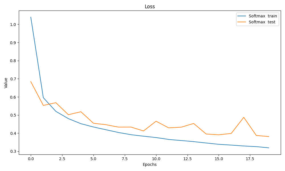
test loss有点鬼畜

其实应该就是在局部最小值震荡了，可能是学习率略高，不过应该不是很影响结果就懒得调了 其实是我水平不行

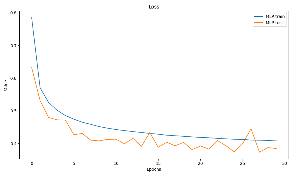
MLP

我们知道，线性模型很好，但是可惜现实总是很骨感，大部分事情都是非线性的。那么我们如何去拟合非线性呢？这需要我们用到MLP多层感知机。

其实MLP的核心就是一个非线性的激活函数。激活函数有很多，我不一一列举，本次训练使用的是relu函数

定义net

    net = nn.Sequential(nn.Flatten(), nn.Linear(num_inputs, num_hidden),
                        nn.ReLU(), nn.Linear(num_hidden, num_outputs))

其实就是用一个激活函数把线性层之间隔开

如果中间没有激活函数，其实就相当于一层，可以想想为什么

定义trainer

trainer1 = torch.optim.SGD(net.parameters(), lr=0.1)

训练

    timer[1], epoch_losses, test_losses = train_net(net, train_iter, num_epochs, loss, trainer1,test_iter)

结果是这样

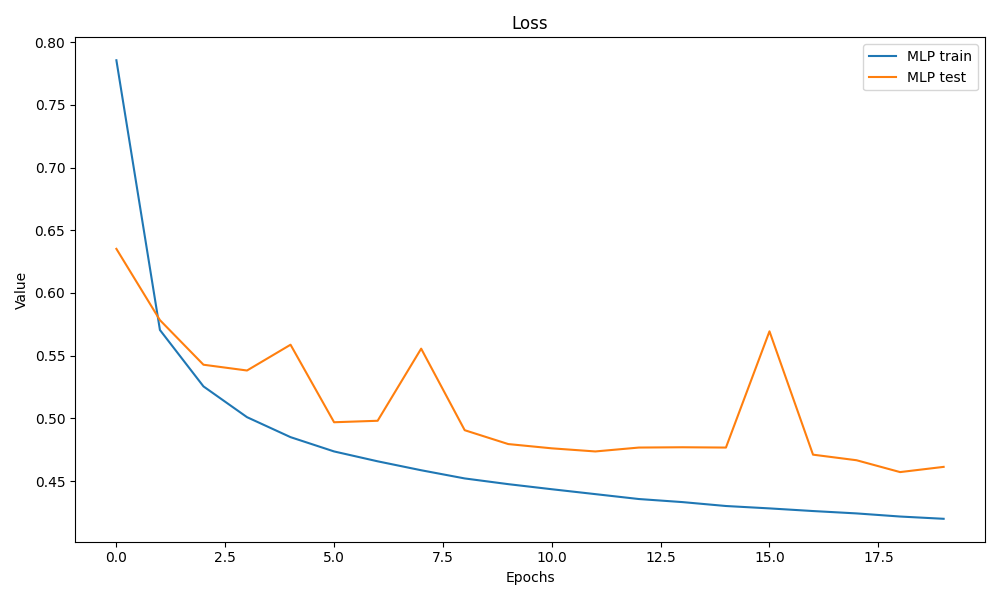
仍然很鬼畜

MLP + 权重衰减

我们也许知道。模型在训练集上拟合的太好并不是一件好事，这意味着模型的抗干扰能力很差，容易学习到一些奇奇怪怪的噪声。其实就是想让训练误差和泛化误差尽量接近。为此，我们需要一些正则化的方法

权重衰减

某个神经元权重过大不是一件好事，因为这意味着我们的模型过于依赖这个神经元，这个位置的输入微小的变化会引起输出的剧烈改变

那么怎么限制权重w的大小呢？我们可以在loss里面增加一个惩罚项
$$
\frac{\lambda}{2}||w||^2
$$
假如w过大，loss就会变大，然后拉着w变小

所以我们的loss变成了这样
$$
loss=LossEntropyLoss+\frac{\lambda}{2}||w||^2
$$
然后接下来

net_weight_decay = nn.Sequential(
        nn.Flatten(),
        nn.Linear(num_inputs, num_hidden),
        nn.ReLU(),
        nn.Linear(num_hidden, num_hidden2),
        nn.ReLU(),
        nn.Linear(num_hidden2, num_outputs),
    )
trainer_weight_decay = torch.optim.SGD(
    net_weight_decay.parameters(), lr=0.1, weight_decay=lambd)

 timer[2], epoch_losses_weight_decay, test_losses_weight_decay = train_net(net_weight_decay, train_iter, num_epochs, loss, trainer_weight_decay,test_iter)

在sgd里面让weight_decay=lambd就会引入权重衰减，不需要写其它的loss 调包就是爽

结果

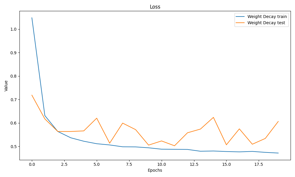
越来越鬼畜

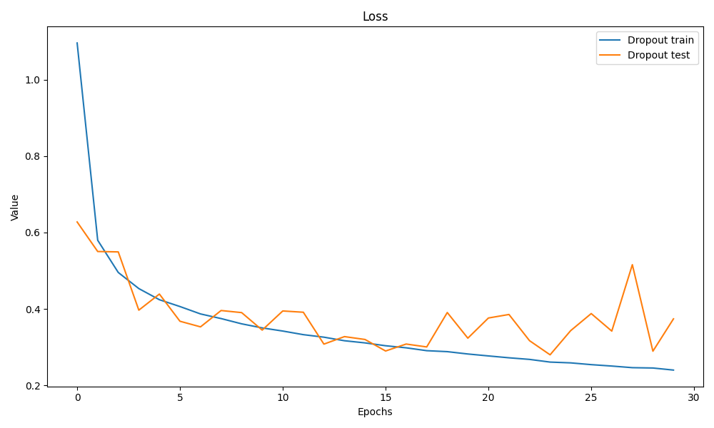
MLP + dropout

关于模型的正则化，其实我们还有一种方法，那就是dropout。它的原理是在把隐藏层随机丢弃一些神经元，然后对应调大其它神经元的输出。这个做法可以防止模型过于依赖某个神经元从而增强泛化性能，防止学习到一些噪声

如果打个比方，可能就像一个公司，平常的时候来一半人也能正常运转，然后来活的时候就全上，这样测试的结果肯定相对好一些

dropout的公式是这样的：
$$
x_i'=
\begin{cases}
0&概率为p\
\frac{x_i}{1-p}&其它情况
\end{cases}
$$
可以计算一下，期望是不变的

接下来，仍然是调包

net_dropout = nn.Sequential(
        nn.Flatten(),
        nn.Linear(num_inputs, num_hidden),
        nn.ReLU(),
        nn.Dropout(0.2),
        nn.Linear(num_hidden, num_hidden2),
        nn.ReLU(),
        nn.Dropout(p),
        nn.Linear(num_hidden2, num_outputs),
    )    

这里第一层dropout的概率是0.2，因为是试验过，如果第一层就0.5效果不好

定义train然后训练

    trainer_dropout = torch.optim.SGD(
        net_dropout.parameters(), lr=lr)

    timer[3], epoch_losses_dropout, epoch_accs_dropout = train_net(net_dropout, train_iter, num_epochs, loss, trainer_dropout,test_iter)

结果是这样

可以看到test loss波动不算太大

附录

附上我调参后跑的几个模型和我的源代码

from re import X
import torch
from torch import  nn
from d2l import torch as d2l
import matplotlib.pyplot as plt
import time
import numpy as np
import torchvision
from torch.utils import data
from torchvision import transforms

def get_dataloader_workers():
    return 4

def init_weights_Kaiming(m):
    if type(m) == nn.Linear:
        nn.init.kaiming_normal_(m.weight, mode='fan_in', nonlinearity='relu')
        nn.init.zeros_(m.bias)

def load_data_fashion_minst(batch_size, resize=None):
    trans = [
        transforms.ToTensor(),
        #transforms.Lambda(lambda x : x.view(-1))
    ]
    if resize:
        if isinstance(resize, (tuple, int)):
            trans.insert(0, transforms.Resize(resize))  # type: ignore
        else:
            raise ValueError(
                "resize must be an integer or a tuple of integers")
    trans = transforms.Compose(trans)
    #    print(trans)
    mnist_train = torchvision.datasets.FashionMNIST(root="data",
                                                    train=True,
                                                    transform=trans,
                                                    download=True)
    mnist_test = torchvision.datasets.FashionMNIST(root="data",
                                                   train=False,
                                                   transform=trans,
                                                   download=True)
    return (data.DataLoader(mnist_train,
                            batch_size,
                            shuffle=True,
                            num_workers=get_dataloader_workers()),
            data.DataLoader(mnist_test,
                            batch_size,
                            shuffle=False,
                            num_workers=get_dataloader_workers()))

def init_weights(m):
    if type(m) == nn.Linear:
        nn.init.normal_(m.weight, std=0.01)
        nn.init.zeros_(m.bias)

def init_zeros(m):
    if type(m) == nn.Linear:
        nn.init.zeros_(m.weight)
        nn.init.zeros_(m.bias)

def train_epoch(net, train_iter, loss, trainer):
    for X, y in train_iter:
        X, y = X.to(next(net.parameters()).device), y.to(
            next(net.parameters()).device)
        y_hat = net(X)
        l = loss(y_hat, y).mean()
        trainer.zero_grad()
        l.backward()
        trainer.step()
    return

class Accumulator:

    def __init__(self, n):
        self.data = [0.0] * n

    def add(self, *args):
        self.data = [a + float(b) for a, b in zip(self.data, args)]

    def __getitem__(self, idx):
        return self.data[idx]

def evaluate_accuracy(net, test_iter):
    if isinstance(net, torch.nn.Module):
        net.eval()
    metric = Accumulator(
        2)  # Sum of correct predictions and total number of predictions
    with torch.no_grad():
        for X, y in test_iter:
            X, y = X.to(next(net.parameters()).device), y.to(
                next(net.parameters()).device)
            metric.add(d2l.accuracy(net(X), y), y.numel())
    return metric[0] / metric[1]

def evaluate_one_epoch_loss(net, test_iter, loss):
    if isinstance(net, nn.Module):
        net.eval()
    metric = Accumulator(2)  # Sum of loss and total number of predictions
    with torch.no_grad():
        for X, y in test_iter:
            X, y = X.to(next(net.parameters()).device), y.to(
                next(net.parameters()).device)
            metric.add(loss(net(X), y).sum(), y.numel())
            break
    return metric[0] / metric[1]

def evaluate_loss(net, test_iter, loss):
    if isinstance(net, nn.Module):
        net.eval()
    metric = Accumulator(2)  # Sum of loss and total number of predictions
    with torch.no_grad():
        for X, y in test_iter:
            X, y = X.to(next(net.parameters()).device), y.to(
                next(net.parameters()).device)
            metric.add(loss(net(X), y).sum(), y.numel())
    return metric[0] / metric[1]

def train_net(net, train_iter, num_epochs, loss, trainer,test_iter):
    print(f"Training {net.__class__.__name__}...")
    timer=0
    start_time = time.time()
    epoch_losses = []
    epoch_accs = []
    test_losses = []
    if isinstance(net, nn.Module):
        net.train()
    for epoch in range(num_epochs):
        metric = Accumulator(3)  # Sum of loss, accuracy and total number of predictions
        for X, y in train_iter:

                X, y = X.to(next(net.parameters()).device), y.to(next(net.parameters()).device)
                y_hat = net(X)
                l = loss(y_hat, y).mean()
                trainer.zero_grad()
                l.backward()
                trainer.step()

                # 记录损失和准确率
                metric.add(l.item() * y.size(0), d2l.accuracy(y_hat, y), y.size(0))
                epoch_loss = metric[0] / metric[2]
        epoch_loss = metric[0] / metric[2]
        epoch_acc = metric[1] / metric[2]
        epoch_losses.append(epoch_loss)
        epoch_accs.append(epoch_acc)
        test_losses.append(evaluate_one_epoch_loss(net,test_iter,loss))
    end_time = time.time()
    timer += end_time - start_time

    return timer, epoch_losses, test_losses

def plot_evaluation(test_acc, test_loss, timer, model_names):

    metrics = [test_acc, test_loss]
    metrics_names = ['Accuracy', 'Loss']
    num_models = len(model_names)
    num_metrics = len(metrics)

    bar_width = 0.25
    x = np.arange(0, num_models)
    offsets = [-bar_width, 0, bar_width]
    colors = ['b', 'g', 'r']
    #
    plt.figure(figsize=(10, 6))
    for i in range(num_metrics):
        bars=plt.bar(x + offsets[i],
                metrics[i],
                width=bar_width,
                color=colors[i],
                label=metrics_names[i])
        for bar in bars:
            height = bar.get_height()
            plt.text(bar.get_x() + bar.get_width() / 2.,
                     height + 0.01,  # 稍微高于柱子顶部
                     f"{height:.2f}",  # 显示2位小数
                     ha='center',      # 水平居中
                     va='bottom',      # 垂直底部对齐
                     fontsize=9) 
    plt.xticks(x, model_names)
    plt.xlabel('Models')
    plt.ylabel('Value')
    plt.title('Model Evaluation')
    plt.legend()
    plt.tight_layout()

def plot_training_time(timer, model_names):
    bar_width = 0.15  # Adjust bar width to make bars narrower
    plt.figure(figsize=(10, 6))
    plt.bar(model_names, timer, width=bar_width, color='b')
    plt.xlabel('Models')
    plt.ylabel('Training Time (seconds)')

    plt.title('Training Time per Model')
    plt.xticks(rotation=45)
    plt.tight_layout()

def plot_epoch(epoch_losses, test_loss, model_names):
    plt.figure(figsize=(10, 6))
    plt.plot(epoch_losses, label=f'{model_names} train')
    plt.plot(test_loss, label=f'{model_names} test')
#    plt.ylim(0, 1)
    plt.xlabel('Epochs')
    plt.ylabel('Value')
    plt.title('Loss')
    plt.legend()
    plt.tight_layout()

if __name__ == '__main__':
#    device = torch.device('cuda' if torch.cuda.is_available() else 'cpu')
    device = torch.device('cpu')
    batch_size, lr, num_epochs, num_inputs, num_hidden, num_outputs = 256, 0.1, 30, 784, 256, 10
    num_hidden2 = 256
    p=0.5
    lambd = 0.0005
    net = nn.Sequential(nn.Flatten(), nn.Linear(num_inputs, num_hidden),
                        nn.ReLU(), nn.Linear(num_hidden, num_outputs))
    net = net.to(device)
    net_adam = nn.Sequential(
        nn.Flatten(),
        nn.Linear(num_inputs, num_hidden),
        nn.ReLU(),
        nn.Linear(num_hidden, num_outputs),
    )

    net_adam = net_adam.to(device)

    net_softmax = nn.Sequential(nn.Flatten(),
                                nn.Linear(num_inputs, num_outputs))

    net_softmax = net_softmax.to(device)

    net_4 = nn.Sequential(
        nn.Flatten(),
        nn.Linear(num_inputs, 512),
        nn.ReLU(),
        nn.Linear(512, num_hidden),
        nn.ReLU(),
        nn.Linear(num_hidden, 128),
        nn.ReLU(),
        nn.Linear(128, num_outputs),
    )

    net_4 = net_4.to(device)

    net_weight_decay = nn.Sequential(
        nn.Flatten(),
        nn.Linear(num_inputs, num_hidden),
        nn.ReLU(),
        nn.Linear(num_hidden, num_hidden2),
        nn.ReLU(),
        nn.Linear(num_hidden2, num_outputs),
    )
    net_weight_decay = net_weight_decay.to(device)

    net_dropout = nn.Sequential(
        nn.Flatten(),
        nn.Linear(num_inputs, num_hidden),
        nn.ReLU(),
        nn.Dropout(0.2),
        nn.Linear(num_hidden, num_hidden2),
        nn.ReLU(),
        nn.Dropout(p),
        nn.Linear(num_hidden2, num_outputs),
    )    

    loss = nn.CrossEntropyLoss(reduction='none')
    trainer1 = torch.optim.SGD(net.parameters(), lr=0.1)
    trainer2 = torch.optim.Adam(net_adam.parameters(), lr=lr)
    trainer3 = torch.optim.SGD(net_softmax.parameters(), lr=0.1)
    trainer4 = torch.optim.SGD(net_4.parameters(), lr=lr)
    trainer_weight_decay = torch.optim.SGD(
        net_weight_decay.parameters(), lr=0.1, weight_decay=lambd)
    trainer_dropout = torch.optim.SGD(
        net_dropout.parameters(), lr=lr)

    net.apply(init_weights)
    net_adam.apply(init_weights)
    net_softmax.apply(init_weights)
    net_4.apply(init_weights)
    #net_4.apply(init_weights_Kaiming)

    print("net device:", next(net.parameters()).device)
    print("net_adam device:", next(net_adam.parameters()).device)
    print("net_softmax device:", next(net_softmax.parameters()).device)
    print("net_4 device:", next(net_4.parameters()).device)
    print("net_weight_decay device:", next(net_weight_decay.parameters()).device)
    print("net_dropout device:", next(net_dropout.parameters()).device)
    # Load the data
    train_iter, test_iter = load_data_fashion_minst(batch_size)

    timer = [0.0, 0.0, 0.0, 0.0]  # Initialize timers for each model

    print('Training...\n')

    timer[0], epoch_losses_softmax, test_losses_softmax = train_net(net_softmax, train_iter, num_epochs, loss, trainer3,test_iter)
    timer[1], epoch_losses, test_losses = train_net(net, train_iter, num_epochs, loss, trainer1,test_iter)
#    timer[3], epoch_losses_4, epoch_accs_4 = train_net(net_4, train_iter, num_epochs, loss, trainer4)
    timer[2], epoch_losses_weight_decay, test_losses_weight_decay = train_net(net_weight_decay, train_iter, num_epochs, loss, trainer_weight_decay,test_iter)
    timer[3], epoch_losses_dropout, test_losses_dropout = train_net(net_dropout, train_iter, num_epochs, loss, trainer_dropout,test_iter)
    print('Training complete\n')
    print('Training time:', timer)

    test_acc = [
        evaluate_accuracy(net_softmax, test_iter),
        evaluate_accuracy(net, test_iter),
        evaluate_accuracy(net_weight_decay, test_iter),
        evaluate_accuracy(net_dropout, test_iter),
    ]

    test_loss = [
    evaluate_loss(net_softmax, test_iter, loss),  # 直接计算最终测试损失
    evaluate_loss(net, test_iter, loss),
    evaluate_loss(net_weight_decay, test_iter, loss),
    evaluate_loss(net_dropout, test_iter, loss),
    ]

    # print('Test accuracy:', test_acc)
    # print('Test loss:', test_loss)
    model_names = [
        'Softmax ', 'MLP', 'Weight Decay', 'Dropout'
    ]

    plot_epoch(epoch_losses, test_losses, model_names[0])
    plot_epoch(epoch_losses_softmax, test_losses_softmax, model_names[1])
    plot_epoch(epoch_losses_weight_decay, test_losses_weight_decay, model_names[2])
    plot_epoch(epoch_losses_dropout, test_losses_dropout, model_names[3])

    plot_evaluation(test_acc, test_loss, timer, model_names)
    plot_training_time(timer, model_names)
    plt.show()
#end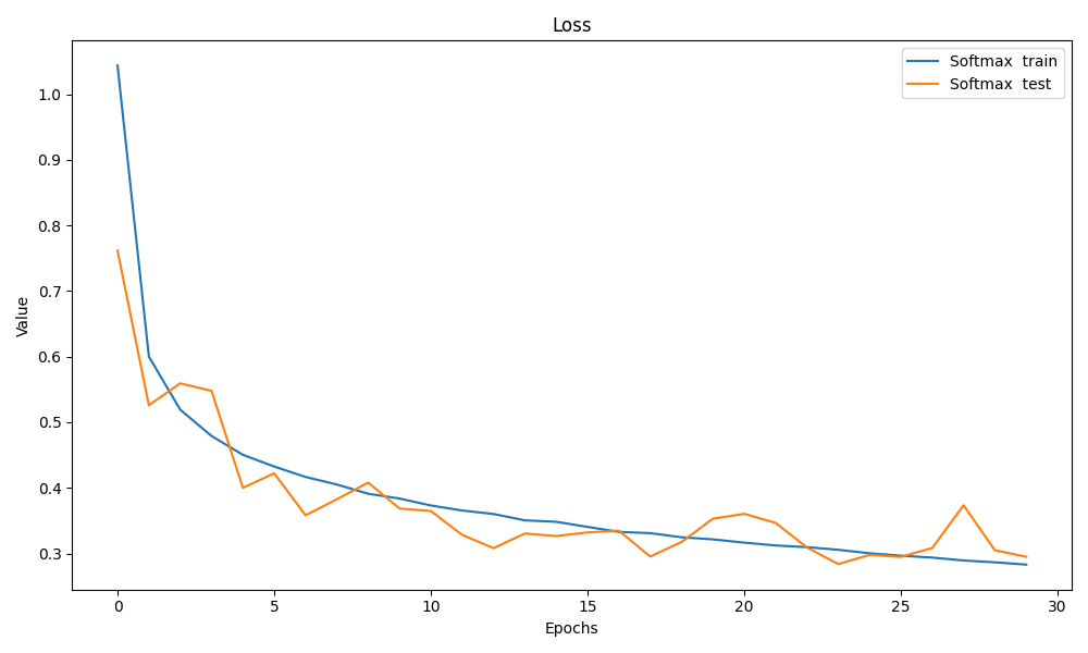

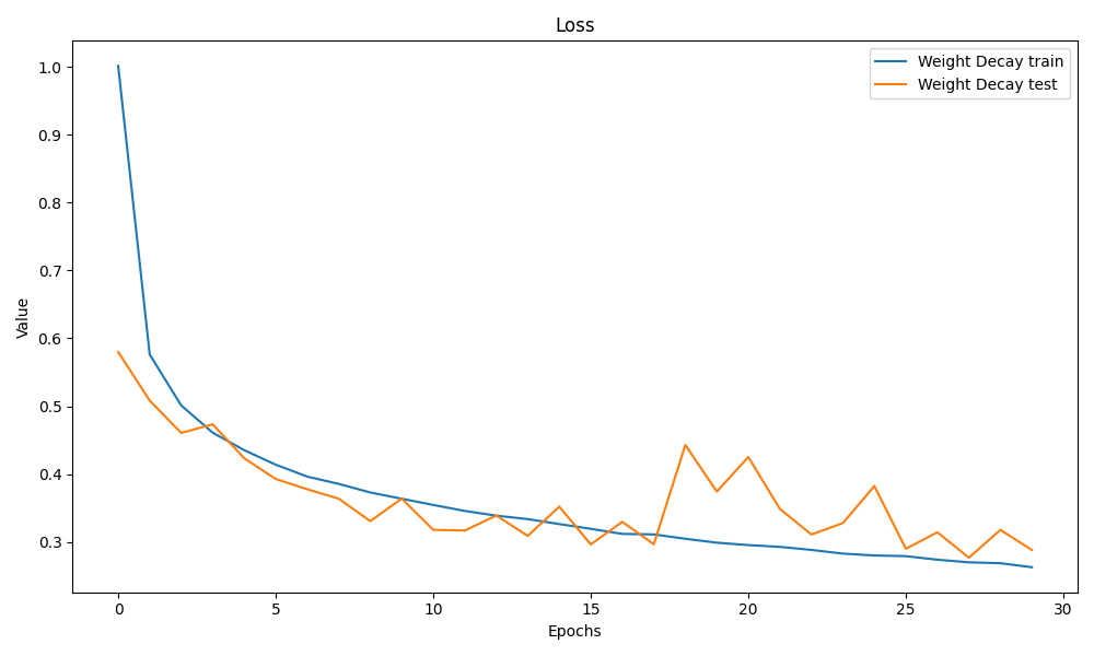
其实就调了权重衰减的参数，20个epoch和30个epoch差别感觉不大

Reference

• 《动手深度学习》第四章 - 李沐